Sampling and statistics: Introduction
Contents
Sampling and statistics: Introduction
Key concepts
types of data
types of error
mean
variance
normal distribution
skewed distribution
standard deviation
standard error
Reading
Glover, Jenkins and Doney – Modeling Methods (GJD)
Sections 2.1-2 - Measurement Theory
Statistical Thinking for the 21st Century (ST21):
Chapter 1: Introduction
Chapter 2: Working with data
Chapter 4: Summarizing data
Focus questions
What is the difference between accuracy and precision?
What are sources of error in the data you work with?
What is the difference between the standard deviation and standard error?
Types of Data
Discrete - represented by an integer (whole number)- counts, presence/absence
Continuous - represented by real1 numbers (e.g. temperature, wave speed, length of an organism, concentration)
Categorical - examples: species, sediment type, hair color, site #
Metadata - “data describing data”
1 Actually, vectors can be represented as complex numbers with an imaginary part
Types of Measurements
Nominal - categories of equal rank
Species Description (phytoplankton types: diatoms, coccolithophores, etc.)
Ordinal - Categories have a logically defined rank. Steps arent equal in size or quantifiable
How sediment grains are categorized: angularity and sphericity
Hurricane scale: ranking is not equivalent to strength
Beaufort Wind Scale: Mariner estimate of wind from wave climate, logically defined, but not quantifiable
Scale: interval and ratio
interval scale: constant succesive intervals, but the reference point is arbitrary e.g. temperature scale
ratio scale: natural zero point (ex: length, mass)
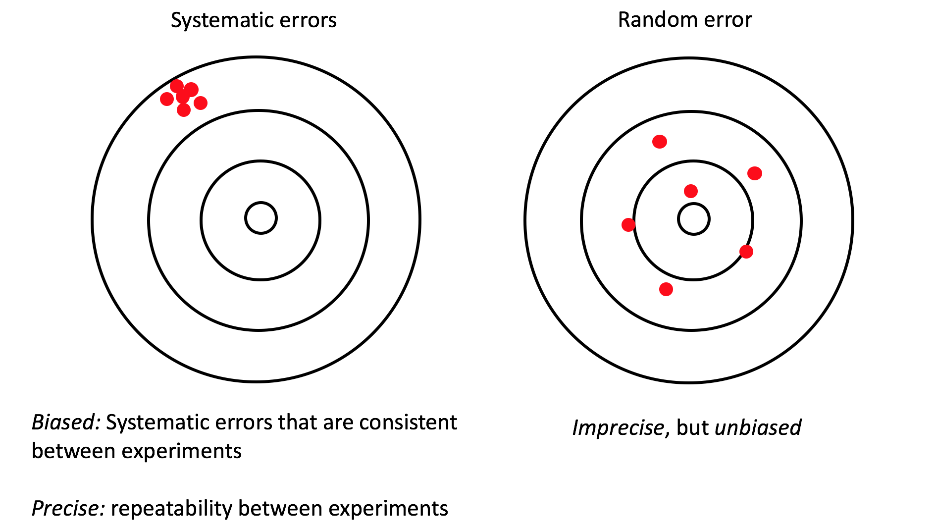
Types of Error
Systematic error - systematically repeatable biased, i.e. some pattern in how they vary
Random error - Impercise, but unbiased. Noise.
Measurement precision
You would not record a value from a ruler to 3.7567453 cm if your ruler only has mm hash marks
Rounding introduces error into your calculations, so in general it is better to use all of the digits that you have and round off to the significant digit when reporting the value
Drift - a systematic error that changes over time

Johnson, K. S., and L. J. Coletti, 2002: In situ ultraviolet spectrophotometry for high resolution and long-term monitoring of nitrate, bromide and bisulfide in the ocean. Deep Sea Res. Part I Oceanogr. Res. Pap., 49, 1291–1305, doi:10.1016/S0967-0637(02)00020-1.
Bottle data (squares): chemically derived values of nitrate (low resolution, high precision)
ISUS Nitrate Sensor (High resolution, systematic error (underreported values compared to bottle casts) , instrument noise (small scale random error))
Smoothing reduces noise, but there is a trade-off: lowers resolution
In this example, the bias is reduced by correcting for the temperature dependence of the sensor.
Sample distributions, probability density
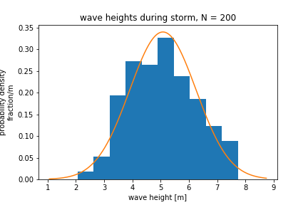
Bars: Example distribution of wave heights during an extreme wave event (N = 200). Synthetic (computer-generated) data based on a similar data set in Emery and Thomson, Section 3.8.4. The sample mean \(\bar{x}\) is 5.08 m and the sample standard deviation \(s\) is 1.18 m.
Wave height categories are divided in to bins of with \(\Delta x\)
Probability density = fraction/\(\Delta x\)
Orange line: Normal distribution (hypothetical), allows the use of mathematical theories to use statistics. The shape of the normal distribution is defined by two parameters - the mean and standard deviation. This theoretical curve has the same mean and standard deviation as the sample distribution.
Integral of area under the curve = 1 (all probability falls under the curve) for both the sample distribution and the theoretical normal distribution.
Cumulative distribution
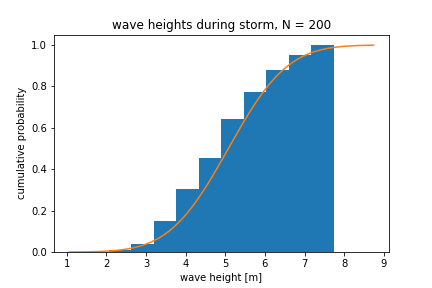
Same samples and theoretical probability, expressed as cumulative probability. This is the probability that the data fall with a given interval or less.
Descriptive statistics
Mean
With a finite number of \(N\) samples, the true mean of a population, \(\mu\) (“mu”), can be estimated by the sample mean \(\bar{x}\),
Variance
Variance describes the spread of the data. The sample variance is equal to the sample standard deviation squared (\(s^2\)). The sample variance is an estimate of the true variance (\(\sigma^2\))
where \(N-1\) is the degrees of freedom. Degrees of freedom are the number of independent pieces of information. The variance of one sample (\(N=1\)) is essentially meaningless because it is always equal to zero, no matter what the value of the sample is. In this case, there are no degrees of freedom. Calculating the variance/standard deviation with \(N-1\) in the denominator is called the unbiased estimate of the true standard deviation \(\sigma\).
The variance is positive definite because it is the sum of squared values and therefore cannot be negative.
Standard Error
The standard error describes how well the sample mean describes the true mean
The standard error does not describe the spread of the data, it describes the how well the sample mean, \(\bar{x}\), represents the true mean, \(\mu\). The standard error can thought of as an estimate of the standard deviation of \((\bar{x} - \mu)\), after many repeated experiments with \(N\) samples.
Example revisited: repreated trials
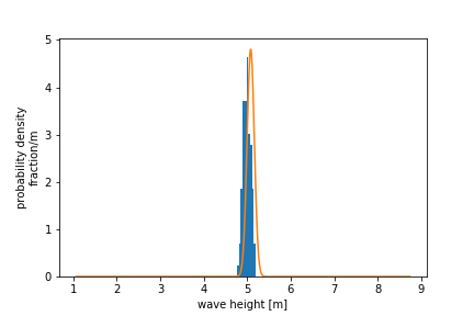
Results from 100 repeated trials during same storm (N = 200 each trial). The \(x\)-axis is the same as that shown for the sample distribution above, to emphasize how the distribution of means clusters more tightly together. We can think of these repeated trials as different instruments measuring different waves in the same storm. Note that this is easy to do with a computer-generated example dataset, but not so easy to do in practices.
Blue bars: Probability density of the mean of each trial (mean of all sample means = 4.99m)
Orange curve: Normal distribution Mean = Mean of trial 1 (example distribution shown above). Standard deviation = Standard error of trial 1, SE = \(s/\sqrt{N}\)
The standard error from 1 set of samples, gives an estimate of standard deviation (spread) of the means.
Programming tutorial: Unix shell
See notes on the Software Carpentry website.