Modeling, sampling, confidence intervals
Contents
Modeling, sampling, confidence intervals
Recommended reading
http://statsthinking21.org/index.html Chapters 7,8
Glover, Jenkins and Doney: Section 2.7 - The central limit theorem
Emery and Thomson: Confidence intervals, 3.8.1, 3.8.2 – Confidence interval for mean
Probability Density Function (PDF) review with example data set
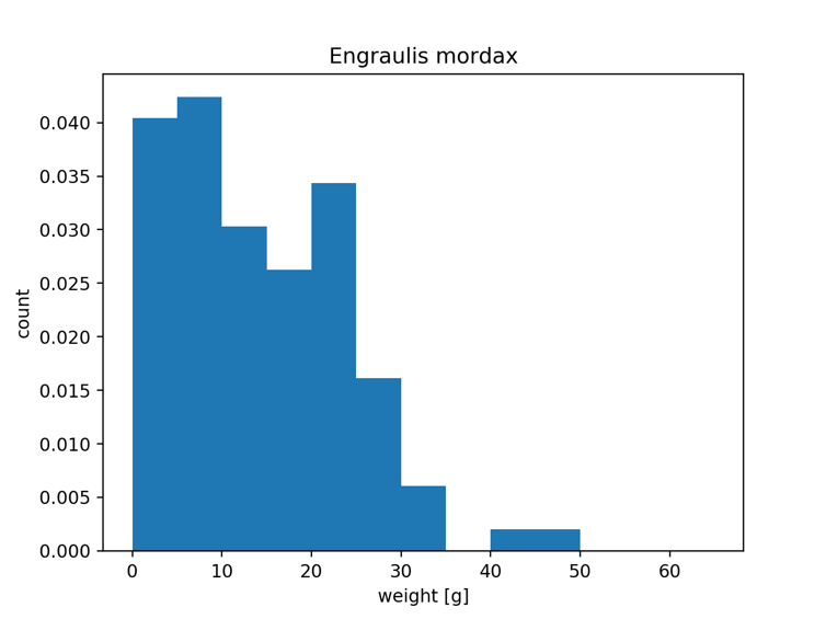
Probability density function
\(N\) = 10623 anchovy weight samples
\(\Delta x\) = 5 g
Review: How to calculate PDF from counts, N and \(\Delta x\) ?
With the histogram we have the following information: counts, bin width ( \(\Delta x\) = 5g), \(N\) (samples).
PDF = fraction/\(\Delta x\) = counts/(\(N \Delta x\))

NOAA SWFSC - Trawl Life History Specimen Data
fishery independent trawl surveys of coastal pelagic species
Surveys: 2003-2019
Subsampled data set
N = 100 anchovy weight samples
What are the key differences, similarities of distribution, compared with all 10623 samples?
differences: a pdf of smaller sample sizes are noiser, less smooth. May see more variability from one bin to the next.
similarities: theoretical distribution resembles poisson distribution (skewed data set with a longer tail), scale of y-axis (normalized by the bin width so magnitudes of different data sets are comparable)
Statistical modeling
What is a model? - physical models (of a building, of monterey bay, of a cell or a molecule). The general characteristics of a physical model is able to represent something on a different scale to make it easier to understand, to convey the essence of what you are model without having to worry about all the details. a statistical model is same basic idea as a physical model, we want to convey the essence of the dataset without having to use an entire dataset
basic structure of a statistic model - statistical model is based off data
data = model + error
one of the key goals is to quantify that error
Example data set: simplest model
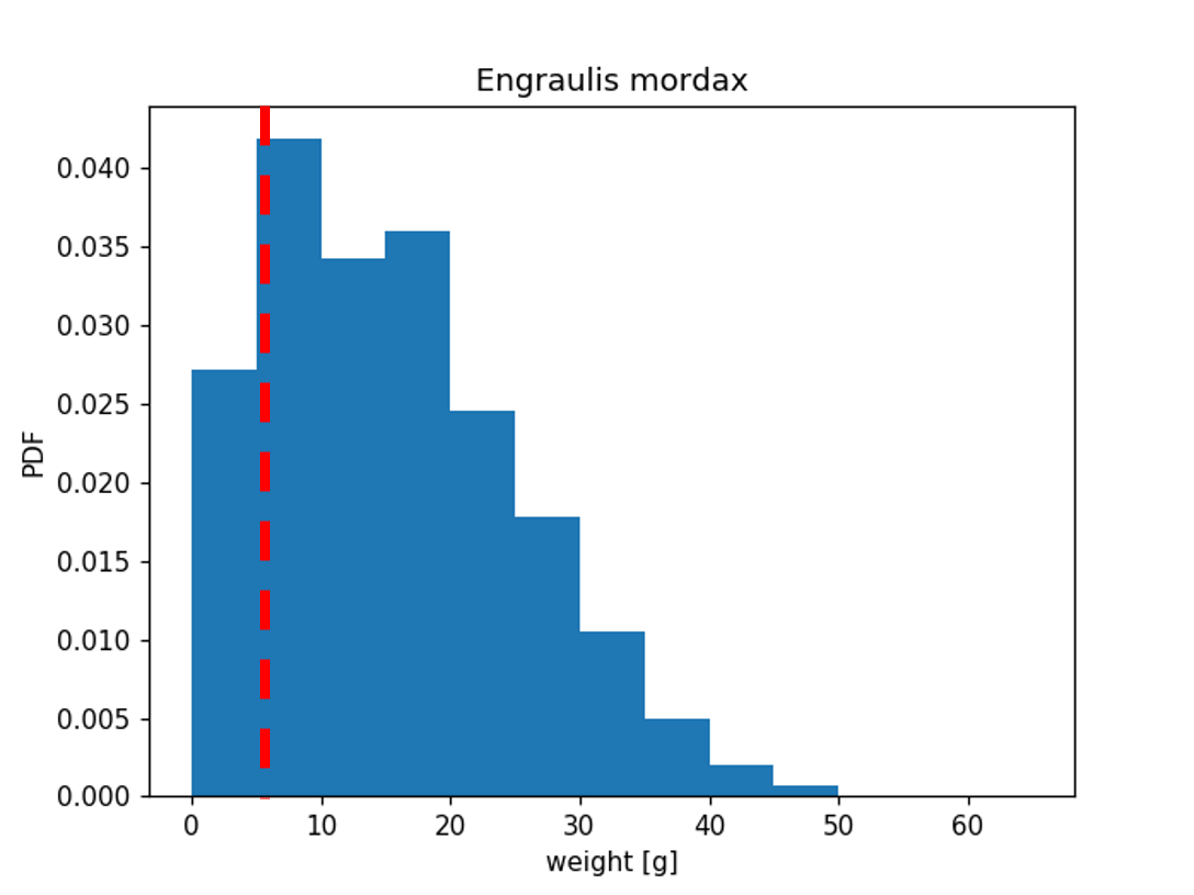
The simplest possible model is a single value
Mode = 5 g
Mean = 15.326 g
Median = 14 g
In this case the mean is much bigger than the mode is about 15 grams (data is skewed). A median describes the central value, or 50th percentile in the data set.
If we use the mode as the model, we can write it as: \(\hat{weight_i}\) = 5 g
\(\hat{}\) denotes a value predicted by the model
\(_i\) is a data point with the model value, a generic observation. If it were a subset of 1, it could mean the first row in a spreadsheet, or 2 meaning the second row, etc.
We can describe the error based on the model structure: \(error_i = weight_i - \hat{weight_i}\)
Each observation has a model value and an error associated with it.
\(weight_i\) is an observation, or data point
In the example, if we have 10K data points, then we have 10k errors.
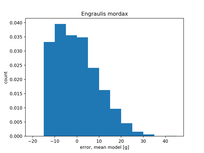
Example data set: mode as a model
Average error when using mode as model: 10.326 g
If we use the mean as a model, will the average error increase or decrease?
Example data set: mean as a model
If we use the mean as a model, \(\hat{x_i} = \bar{x_i}\)
The average error when using mean as a model is 0.0g. In this case, the negative errors cancel out the positive errors, and in this case, using the mean as a model does not best describe the data.
What other metrics can we use to quantify model error?
Some ways of quantifying the error:
We can describe the mean error (average error) as:
\(ME = \frac{1}{N} \sum_{i=1}^N (x_i - \hat{x_i})\)
If our model (\(\hat{x_i}\)) is the mean of the dataset (\(\bar{x_i}\)), then the ME = 0 and is unbiased.
Sum of Squared Errors
\(SSE = \sum_{i=1}^N (x_i - \hat{x_i})^2\)
(This treats the positive and negative values equally)
Mean Squared Error
\(MSE = \frac{1}{N} SSE\)
Root Mean Square Error
\(RMSE = \sqrt{MSE}\)
The units for RMSE will make it easier to understand the error mismatch. This is a summary of all the errors in the dataset by penalizing all errors in the dataset equally.
RMSE(mean) = 9.71 grams (describing the spread or standard deviation of the error)
RMSE(mode) = 14.18 grams (this is biased)
The mean is the single value that minimizes RMSE
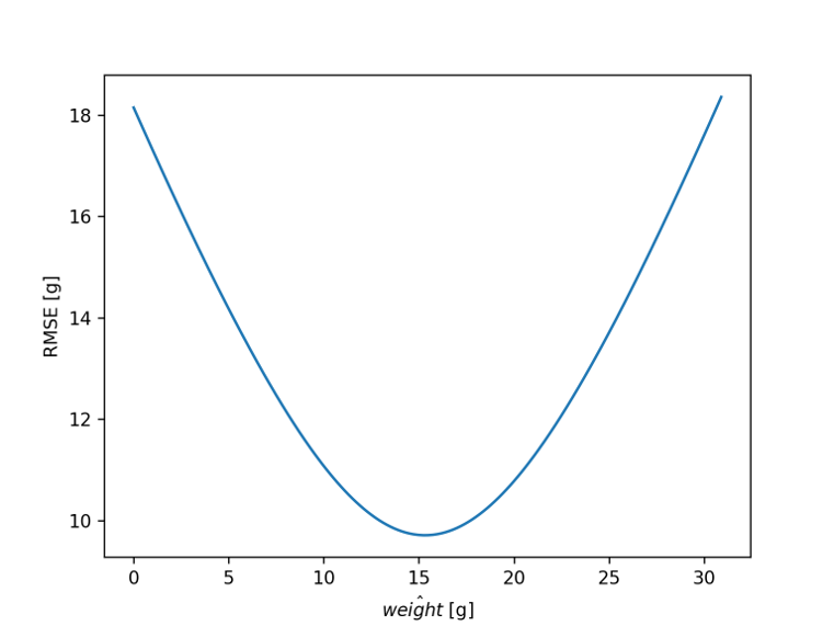
This plot is showing the rmse as a function of the model value. Different models will minimize different types of errors (mean, median, mode).
This plot is called a ‘cost function’ we have a model parameter (x-axis), we have a cost (y-value). The goal of modeling is to minimize the cost function
Example data set: linear model
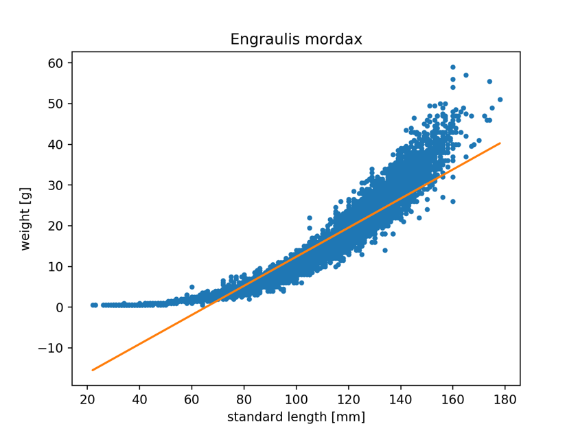
RMSE = 3.57 g
Looking at the data, it looks like a linear model only works for part of the data. If we were going to use this linear model, our equation would be:
\(\hat{weight_i} = constant + a * length_i\)
\(\hat{}\) indicates \({weight_i}\) is a model
constant = the intercept
a = the slope
The intercept and slope are the model parameters. You can think of the error as being the vertical distance between the data point and the model.
Example data set: quadratic model
RMSE = 2.11 g
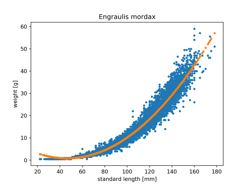
\(\hat{weight_i} = constant + a * length_i + b * length_i^2\)
The constant, a, and b are model parameters that describe the structure or the shape of the model. We can find the model that minimizes the RMSE. This looks like it is doing better than a linear model, but the model indicates that their weight decreases as they get bigger for smaller fish. It still has some systematic errors where there is some bias.
Example data set: data transformation
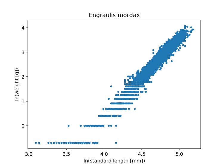
This is the same data transformed to a logarithmic scale, and now it appears that a linear model may be appropriate. Now, we are not minimizing the RMSE, you are minimizing the logarthmic RMSE.
What makes a model good?
good fit
minimizes error
represents actual scenario of the data (think ahead of error sources)
is not overcomplicated
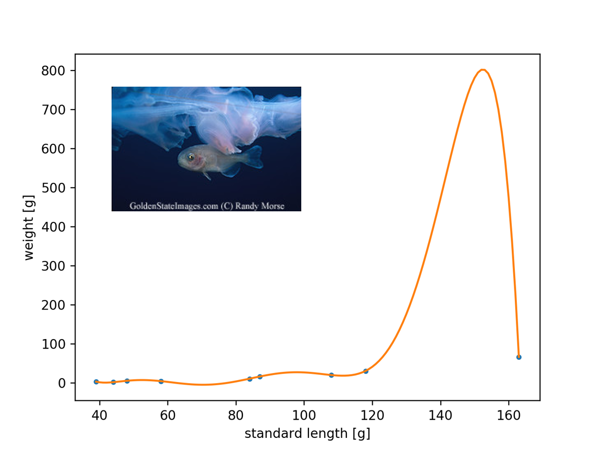
Overfitting
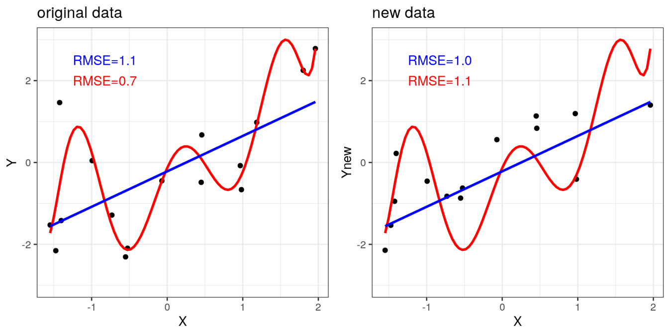
Model is overcomplicated and not representative of the actual scenario. If another datapoint is added not on the model, the RMSE will be huge. More data points will quickly deteriorate the model.
Sampling
Statistical inference: One of the foundational ideas in statistics is that we can make inferences about an entire population based on a relatively small sample of individuals from that population.
Goal of sampling: determine the value of a statistic for an entire population of interest, using just a small subset of the population.
The way in which we select the sample is critical to ensuring that the sample is representative of the entire population.
Adapted from: http://statsthinking21.org/sampling.html
Back to the anchovy data example: distribution of means
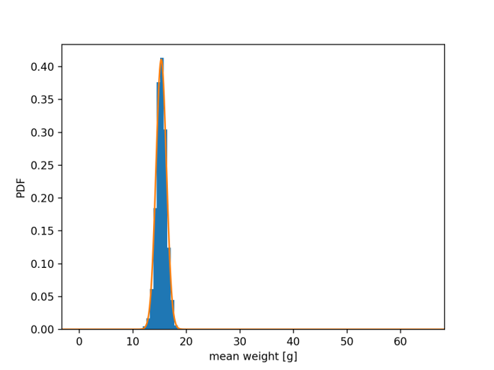
Blue bars: distribution of 1000 different sample means (\(\bar{x}\)), with N = 100 samples each
Mean of \(\bar{x}\) = 15.346 g Std. dev. of \(\bar{x}\) = 0.933 g
Orange curve: normal distribution
\(\mu\) = 15.327 g (mean of full data set)
\(\frac{\sigma}{\sqrt{N}}\) = 0.971 g (std. dev. of full data set / √100)
Anchovy data: distribution of means (zoomed in)
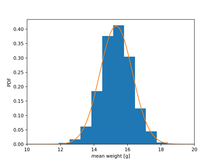
Blue bars: distribution of 106 different sample means (\(\bar{x}\)), with N = 100 samples each
Mean of \(\bar{x}\) = 15.358 g Std. dev. of \(\bar{x}\) = 0.822 g
Orange curve: normal distribution
\(\mu{}\) = 15.327 g (mean of full data set)
\(\frac{\sigma}{\sqrt{N}}\) = 0.971 g (std. dev. of full data set / √100)
This is a consequence of the central limit theorem.
The Central Limit Theorem
The central limit theorem states that no matter what the probability distribution of parent population is, the mean of the means drawn from the same population is normally distributed for large sample sizes. As \(N\) approaches infinity,
mean\((\bar{x}) \rightarrow \mu\) (the mean of the sample means approaches the true mean)
std\((\bar{x}) \rightarrow \frac{\sigma}{\sqrt{N}}\) (the standard deviation of the sample means approaches the true standard error)
The important consequence of this theorem is that if you collect enough samples, the sample mean will always provide an unbiased estimate of the true mean and you can calculate confidence intervals with the formulas above.
However, if you have too few samples, the sample mean will provide a biased estimate.
Some examples of situation where the central limit theorem is applied:
Radiochemists study discrete decay events, which follow a Poisson distribution. A few samples will give a biased estimate of the mean rate of radioactive decay. If enough samples are collected, the sample mean and 95% confidence intervals can be calculated using the formulas described above.
Physical oceanographers routinely take advantage of the central limit theorem when using observations of pressure or velocity measurements to study processes with time scales much longer than individual waves. The probability distribution of a wavy sea surface is not normal at all, but by collecting many samples (a.k.a. and ensemble) over a period of ~10-20 minutes we can effectively “average out” the waves and be confident in the mean of that ensemble.
When sampling a noisy environment and ensemble averaging, oceanographers must be careful to choose an ensemble that is long enough to collect enough samples, but not so long that the statistics are changing significantly over longer time scales. If statistics are robust regardless, of the sampling duration, the process is said to be stationary.
*Adapted from: http://statsthinking21.org/sampling.html
Central limit theorem (in other words)
The distribution of an average tends to be Normal, even when the distribution from which the average is computed is decidedly non-Normal.
http://www.statisticalengineering.com/central_limit_theorem.htm
The amazing and counter-intuitive thing about the central limit theorem is that no matter what the shape of the original distribution, the sampling distribution of the mean approaches a normal distribution. Furthermore, for most distributions, a normal distribution is approached very quickly as N increases.
Central limit theorem - applications
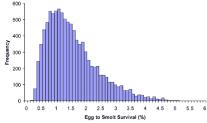
This distribution is skewed, but there are hundreds of samples
The 95% confidence interval for the mean can still be estimated as
\(\bar{x}\) ±1.96 \(\frac{s}{\sqrt{N}}\)
With very few samples, the mean would not only be uncertain, but also biased
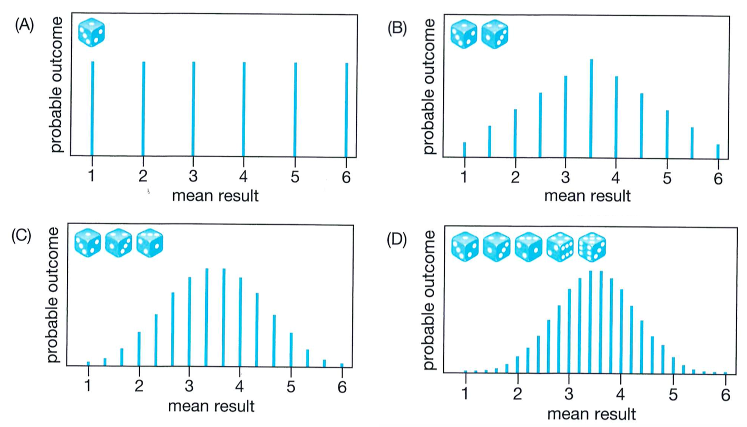
Central limit theorem – dice example
If we start to get more samples, we start to get more of a peak in the distribution
The z Distribution
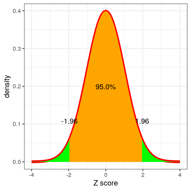
According to the central limit theorem, sample means (\(\bar{x}\)) are normally distributed for large N.
This gives you data that is standardized in a way that if we take z-scores of the sample means (\(\bar{x}\)), 95% of them should fall in the range:
-1.96 < z < 1.96
This is the basis for forming 95% confidence intervals
Confidence intervals for the mean
\(CI_{95\%} = \bar{x} \pm 1.96 \times SE\), where SE is the standard error \(\frac{S}{\sqrt{N}}\)
With large enough sampling size N, the 95% confidence interval will contain the true population mean 95% of the time.*
Common misinterpretation of confidence intervals*:
“There is a 95% chance that the population mean falls within the interval.”
What is wrong with this statement, and how does it differ from the correct interpretation?
In the case of confidence intervals, we can’t interpret them in this wasy because the population parameter has a fixed value - it is or it isn’t in the interval
It is the sample mean that has a probability of falling within the confidence intervals, not the true mean
*Adapted from: http://statsthinking21.org/sampling.html