Multivariate regression
Contents
Multivariate regression
Goal: Find a relationship that explains variable \(y\) in terms of variables, \(x_1, x_2, x_3\),…\(x_n\)
source: http://www.sjsu.edu/faculty/gerstman/EpiInfo/cont-mult.htm
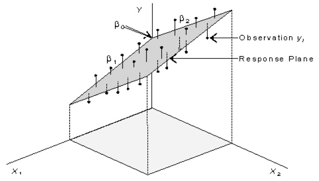
This three dimensional visualization shows how linear model based on two predictor variables, \(x_1\) and \(x_2\) can be used to model a response variable \(y\). A constant and two slopes to define a 2D plane in 3D space. The sum of squared vertical distances between the plane (model) and observations of \(y\) are minimized. Like fitting a line in 2D space, this procedure assumes the validity of a linear model.
Example: Model for aragonite saturation state based on three other oceanographic variables
As a motivation for multiple linear regression, we consider a model for aragonite saturation state, \(\Omega_A\). The study by Juranek et al. (2009), discussed on greater detail below, uses multiple linear regression to model \(\Omega_A\) for surveys where it is not measured, using more commonly measured parameters. We know that \(\Omega_A\) depends on both physical and biological processes, so one candidate for a model might be:
\(y = b_0 + b_1x_1 + b_2x_2 + b_3x_3\)
where \(y\) = \(\Omega_A\)
\(x_1\) = temperature
\(x_2\) = salinity
\(x_3\) = dissolved oxygen
\(k\) = 3 predictor variables
\(N\) = 1011 samples
Because we have three predictor variables, it is hard to visualize in four-dimensional space. However, the same principles are involved as fitting a 1D line in 2D space, or a 2D plane in 3D space.
Equations for linear model
A linear model can be represented as a system of \(N\) equations.
where \(\hat{y}_i\) is a modeled value and \(\epsilon_i\) is the difference between the modeled value, \(\hat{y}_i\) and an observation \(y_i\). The least squares regression minimizes the sum of \(\epsilon_i^2\), the overall deviation between the linear model and data.
Matrix form
To solve a least squares problem numerically, it helps to write the system of equations for the model in matrix form.
Form a vector \(Y\) of \(N\) observations.
A vector \(B\) contains \(k+1\) unknown coefficients.
The predictor variables are stored as columns in a matrix with \(N\) rows and \(k+1\) columns
Now the system of equations for the linear model can be written as
\( X B = Y\)
Numerical solution
The least squares problem is solved using a singular value decomposition method. Efficient alorithms for this procedure are typically included in scientfic computing software. In Python, create an array for the vector \(Y\) and a 2D array for the matrix \(X\). Then use np.linalg,lstsq to solve for \(B\).
import numpy as np
B = np.linalg.lstsq(X,Y)
Testing for significance
F test
Similar to ANOVA significance calculation, which also involves ratios of squared values.
\(H_0 : \hat{y} = C_0\) (All non-constant coefficients are zero)
\(H_1 :\) At least one coefficient is non-zero
Total sum of squares
Regression sum of squares
where \(\hat{y_j}\) are model values
Error sum of squares
F-statistic
Mean squares statistics, calculated by dividing by degrees of freedom:
\(MST =\frac{SST}{N-1}\)
\(MSR =\frac{SSR}{k}\) , where k is the number of variables
\(MSE = \frac{SSE}{N-k-1}\)
\(F = \frac{MSR}{MSE}\)
This test statistic can be compared with a critical F value, which depends on significance level \(\alpha\) and the degrees of freedom in the numerator and denominator. If F is larger, then error is small. Find F using statistical tables, or stats.f.ppf in Python.
Multiple regression example: modeling aragonite saturation state
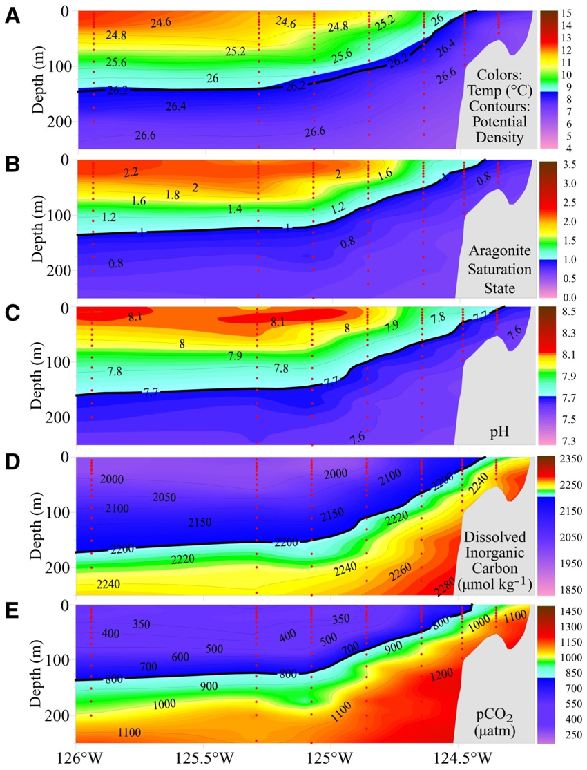
Source: Feeley et al. (2208) Evidence for upwelling of corrosive acidification water onto the continental shelf, Science
At Aragonite staturation state > 1 aragonite (calcium carbonate will dissolve in seawater)
Is there a way to estimate aragonite saturation state \(\Omega_{Ar}\) based on more commonly measured parameters?
Where \(K'_{sp}\) is the stoichiometric solubility product function of T,S,pr and mineral phase (aragonite, calcite)
\([Ca^{2+}]\) doesn’t change much
\([CO_3^{2+}]\) can be calculated from chemical measurements of DIC, \(pCO_2\), total alkalinity and pH (at least two of these 4 parameters).
Models
Juranek et al. (2009) describe a set of least squares regression models for aragonite saturation state, based on more commonly measured oceangraphic variables (temperature, salinity, pressure, oxygen and nitrate).
Juranek, L. W., R. A. Feely, W. T. Peterson, S. R. Alin, B. Hales, K. Lee, C. L. Sabine, and J. Peterson, 2009: A novel method for determination of aragonite saturation state on the continental shelf of central Oregon using multi-parameter relationships with hydrographic data. Geophys. Res. Lett., 36, doi:10.1029/2009GL040778.
Model 1
Has high \(R_a^2\) (“adjusted” \(R^2\))
High “variance inflation factor”
Indicates multiple collinearity
Coefficients are ambiguous and not meaningful - When you add more data, you get will get a different answer (this is bad!)
Adjusted \(R^2\)
Accounts for reduction of degrees of freedom when using multiple predictor variables.
If the MSE is low, the adjusted R-squared is going to be high. The more observations you have, the less this adjustment matters.
Variance Inflation Factor
Variance Inflation Factor
where \(R^2 \) from regression of predictor variables against other predictor variables. There is no clear “cut-off” that defines high VIF, but greater than 5 (and definitely greater than 10) is generally considered high.

Final Model
Less variables, avoids multiple collinearity
Includes interaction term
Reference values (\(T_r\) and \(O_{2,r}\)) keep product from getting too big
Using variables with differing magnitudes can lead to problems like round-off errors
Standardizing variables (using z-scores) another common strategy
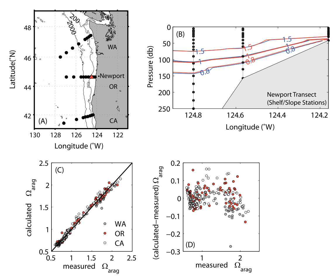
Aragonite saturation state
Red contours: from measured DIC and total alkalinaity
Blue contours: Multiple regression model
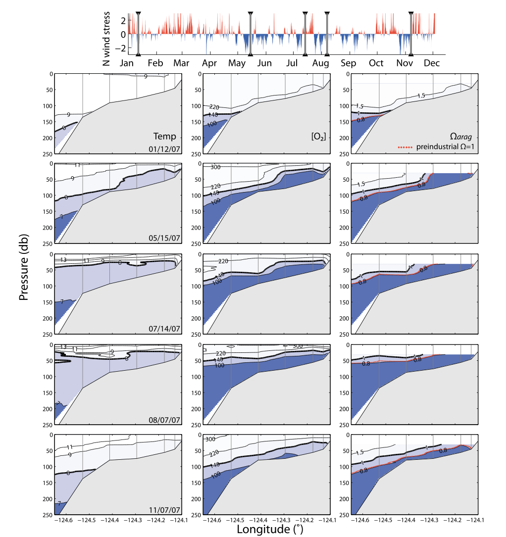
Application of the model to time series that do not have direct observations of the carbonate system parameters