The generalized linear model
Contents
The generalized linear model
Common statistical tests as linear models
Many statistical tests can be though of as implementations of the generalized linear model. Thinking of tests as part of a class of linear models can be more intuitive than thinking about how each test works individually.
Resources
This approach is taken in Chapter 28 of Statistical Thinking for the 21st Century on comparing means:
A blog post by Jonas Kristoffer Lindeløv explains this approach for a wide array of statistical tests. Implementation of the statistical functions and linear models, with interpretations, are provided in both R and Python.
Original post (using R): https://lindeloev.github.io/tests-as-linear/
Python port: https://eigenfoo.xyz/tests-as-linear/
Examples
The following examples show different ways of comparing means, using data from the 2007 West Coast Ocean Acidification cruise. The examples use quality controlled data from 0-10 dbar (upper 10m of the water column).
Comparing two sample means (another example)
The following shows the same calculations for temperature. In this case, the null hypothesis can be rejected at the 95% confidence level, and the 95% confidence intervals for the model slope do not overlap with zero.
Load 2007 data
import numpy as np
import pandas as pd
import matplotlib.pyplot as plt

from scipy import stats
import statsmodels.formula.api as smf
import pingouin as pg

import PyCO2SYS as pyco2
/Users/tomconnolly/programs/miniconda3/envs/data-book/lib/python3.8/site-packages/outdated/utils.py:14: OutdatedPackageWarning: The package pingouin is out of date. Your version is 0.5.0, the latest is 0.5.1.
Set the environment variable OUTDATED_IGNORE=1 to disable these warnings.
  return warn(
filename07 = 'data/wcoa_cruise_2007/32WC20070511.exc.csv'
df07 = pd.read_csv(filename07,header=29,na_values=-999,parse_dates=[[6,7]])
Use the PyCO2SYS package to calculate seawater carbon chemistry parameters.
https://pyco2sys.readthedocs.io/en/latest/
c07 = pyco2.sys(df07['ALKALI'], df07['TCARBN'], 1, 2,
               salinity=df07['CTDSAL'], temperature=df07['CTDTMP'],
                pressure=df07['CTDPRS'])

df07['OmegaA'] = c07['saturation_aragonite']
/Users/tomconnolly/programs/miniconda3/envs/data-book/lib/python3.8/site-packages/autograd/tracer.py:48: RuntimeWarning: invalid value encountered in sqrt
  return f_raw(*args, **kwargs)
/Users/tomconnolly/programs/miniconda3/envs/data-book/lib/python3.8/site-packages/PyCO2SYS/equilibria/p1atm.py:99: RuntimeWarning: invalid value encountered in sqrt
  lnKF = 1590.2 / TempK - 12.641 + 1.525 * IonS ** 0.5
/Users/tomconnolly/programs/miniconda3/envs/data-book/lib/python3.8/site-packages/PyCO2SYS/equilibria/p1atm.py:577: RuntimeWarning: overflow encountered in power
  K1 = 10.0 ** -(pK1)
/Users/tomconnolly/programs/miniconda3/envs/data-book/lib/python3.8/site-packages/PyCO2SYS/equilibria/p1atm.py:583: RuntimeWarning: overflow encountered in power
  K2 = 10.0 ** -(pK2)
/Users/tomconnolly/programs/miniconda3/envs/data-book/lib/python3.8/site-packages/PyCO2SYS/equilibria/p1atm.py:603: RuntimeWarning: overflow encountered in power
  K1 = 10.0 ** -pK1
/Users/tomconnolly/programs/miniconda3/envs/data-book/lib/python3.8/site-packages/PyCO2SYS/equilibria/p1atm.py:611: RuntimeWarning: overflow encountered in power
  K2 = 10.0 ** -pK2
/Users/tomconnolly/programs/miniconda3/envs/data-book/lib/python3.8/site-packages/PyCO2SYS/equilibria/p1atm.py:636: RuntimeWarning: overflow encountered in power
  K1 = 10.0 ** -pK1
/Users/tomconnolly/programs/miniconda3/envs/data-book/lib/python3.8/site-packages/PyCO2SYS/equilibria/p1atm.py:641: RuntimeWarning: overflow encountered in power
  K2 = 10.0 ** -pK2
/Users/tomconnolly/programs/miniconda3/envs/data-book/lib/python3.8/site-packages/PyCO2SYS/equilibria/p1atm.py:653: RuntimeWarning: overflow encountered in power
  K1 = 10.0 ** -pK1
/Users/tomconnolly/programs/miniconda3/envs/data-book/lib/python3.8/site-packages/PyCO2SYS/equilibria/p1atm.py:658: RuntimeWarning: overflow encountered in power
  K2 = 10.0 ** -pK2
/Users/tomconnolly/programs/miniconda3/envs/data-book/lib/python3.8/site-packages/PyCO2SYS/equilibria/p1atm.py:715: RuntimeWarning: overflow encountered in power
  K2 = 10.0 ** -pK2
/Users/tomconnolly/programs/miniconda3/envs/data-book/lib/python3.8/site-packages/PyCO2SYS/solubility.py:41: RuntimeWarning: overflow encountered in power
  KAr = 10.0 ** logKAr  # this is in (mol/kg-SW)^2
/Users/tomconnolly/programs/miniconda3/envs/data-book/lib/python3.8/site-packages/PyCO2SYS/solubility.py:25: RuntimeWarning: overflow encountered in power
  KCa = 10.0 ** logKCa  # this is in (mol/kg-SW)^2 at zero pressure
Comparing two sample means (another example)
The following shows the same calculations for temperature. In this case, the null hypothesis can be rejected at the 95% confidence level, and the 95% confidence intervals for the model slope do not overlap with zero.
Comparing one sample mean to a single value
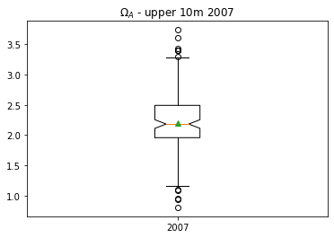
In this example the goal is to test whether the mean aragonite saturation state is different from a value of 1, a critical threshold for the ability of organisms to form calcium carbonate shells.
\(H_0\): \(\bar{\Omega}_A =\) 1
\(H_A\): \(\bar{\Omega}_A \neq\) 1
The first step is to create a subset of good data from the upper 10m.
iisurf07 = ((df07['CTDPRS'] <= 10) &
      (df07['NITRAT_FLAG_W'] == 2) & (df07['PHSPHT_FLAG_W'] == 2)
      & (df07['CTDOXY_FLAG_W'] == 2) & (df07['CTDSAL_FLAG_W'] == 2)
        & (df07['ALKALI_FLAG_W'] == 2) & (df07['TCARBN_FLAG_W'] == 2))

df07surf = df07[iisurf07]
A box plot is one way of showing the distribution of \(\Omega_A\) values.
Orange line: median, or 50th percentile
Upper/lower limits on box: interquartile range, or 75th/25th percentiles
Whiskers: each have length 1.5*interquartile range (pyplot default)
Circles: extreme values
Green triangle: mean
Notches on box: 95% confidence intervals for median
plt.figure()
plt.boxplot(np.array(df07['OmegaA'][iisurf07]),labels=['2007'],showmeans=True,notch=True);
plt.title('$\Omega_A$ - upper 10m 2007')
Text(0.5, 1.0, '$\\Omega_A$ - upper 10m 2007')
Method 1: one sample t-test
A one-sample t-test can be used to test whether the null hypothesis can be rejected at the 95% confidence level (\(\alpha\) = 0.05).
stats.ttest_1samp(np.array(df07surf['OmegaA']),popmean=1)
Ttest_1sampResult(statistic=27.742288359723034, pvalue=4.457126416644256e-58)
Method 2: generalized linear model
Alternatively, this test can be framed in terms of a general linear model
In this application, \(y\) represents the \(\Omega_A\) data. There is only one group, so we can set \(x = 0\) for all values, making the slope parameter \(\hat{a}_2\) irrelevant. The model then reduces to
or a model for the intercept parameter only. This equation can also be expressed as
This model for the data in terms of a constant intercept can be implemented with the statsmodels library:
res = smf.ols(formula="OmegaA ~ 1", data=df07surf).fit()
The summary of the results shows that the intercept is 2.33, which is also the mean of the data. The 95% confidence intervals do not overlap with 1, which means that the null hypothesis can be rejected at \(\alpha\) = 0.05. This approach to hypothesis testing will give the same results as the one sample t-test for \(N\) > 14.
Notice that the test statistic \(t\) is different from the one sample t-test. This is because statsmodels automatically tests whether parameters are different from zero, while in this case we are interested in whether the mean/intercept is different from one.
res.summary()
| Dep. Variable: | OmegaA | R-squared: | 0.000 |
|---|---|---|---|
| Model: | OLS | Adj. R-squared: | 0.000 |
| Method: | Least Squares | F-statistic: | nan |
| Date: | Tue, 03 May 2022 | Prob (F-statistic): | nan |
| Time: | 19:03:38 | Log-Likelihood: | -102.08 |
| No. Observations: | 138 | AIC: | 206.2 |
| Df Residuals: | 137 | BIC: | 209.1 |
| Df Model: | 0 | ||
| Covariance Type: | nonrobust |
| coef | std err | t | P>|t| | [0.025 | 0.975] | |
|---|---|---|---|---|---|---|
| Intercept | 2.2017 | 0.043 | 50.827 | 0.000 | 2.116 | 2.287 |
| Omnibus: | 7.228 | Durbin-Watson: | 0.655 |
|---|---|---|---|
| Prob(Omnibus): | 0.027 | Jarque-Bera (JB): | 11.596 |
| Skew: | 0.177 | Prob(JB): | 0.00303 |
| Kurtosis: | 4.375 | Cond. No. | 1.00 |
Notes:
[1] Standard Errors assume that the covariance matrix of the errors is correctly specified.
Comparing two sample means
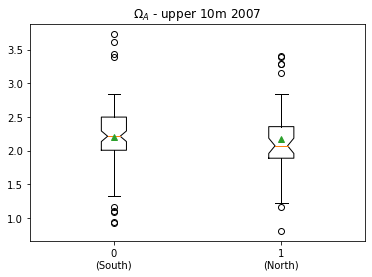
We can also apply the generalized linear model approach when comparing two means. In this case, we will examine whether there is a statistically significant difference between the mean of \(\Omega_A\) to the north and south of Cape Mendocino. At a latitude of 40.4\(^o\)N, Cape Mendocino represents a sharp transition point in many oceanographic processes and water masses.
The first steps are to make two subsets based on latitude, and then visualize the results in a box plot.
# create a new boolean variable in the df07surf dataframe
df07surf = df07[iisurf07]
df07surf = df07surf.assign(is_northern = df07surf['LATITUDE'] > 40.4);

iinorth = np.array(df07surf.is_northern == True)
iisouth = np.array(df07surf.is_northern == False)
plt.figure()
plt.boxplot([df07surf['OmegaA'][iisouth],df07surf['OmegaA'][iinorth]],
            labels=['0\n(South)','1\n(North)'],showmeans=True,notch=True)
plt.title('$\Omega_A$ - upper 10m 2007')
Text(0.5, 1.0, '$\\Omega_A$ - upper 10m 2007')
Method 1: t-test
There is a difference of 0.104 in the mean of \(\Omega_A\) between the two regions.
np.mean(df07surf['OmegaA'][iinorth]) - np.mean(df07surf['OmegaA'][iisouth])
-0.03056105006487364
Is this difference statistically significant? A Student’s t-test can be used to test whether the null hypothesis of no difference can be rejected at the 95% confidence level.
stats.ttest_ind(df07surf['OmegaA'][iinorth],df07surf['OmegaA'][iisouth],equal_var=True)
Ttest_indResult(statistic=-0.3235609219137568, pvalue=0.7467674907175257)
A Welch’s t-test relaxes the assumption of equal variance.
stats.ttest_ind(df07surf['OmegaA'][iinorth],df07surf['OmegaA'][iisouth],equal_var=False)
Ttest_indResult(statistic=-0.30410900939221397, pvalue=0.7619693293723315)
Method 2: generalized linear model
This test can also be framed in terms of a general linear model
Again, \(\hat{y}\) is a model for the aragonite saturation state data. In this case, we can think of the southern data points as having \(x = 0\) and the northern data points as having \(x = 1\).
In this model, the intercept parameter \(\hat{a}_1\) is the mean of the points with \(x = 0\), the southern points.
The slope parameter \(\hat{a}_2\) is equal to the difference between the means of the two groups.
res = smf.ols(formula="OmegaA ~ is_northern", data=df07surf).fit()
The results are summarized below. The slope parameter \(\hat{a}_2\) in our model is the coefficient for the is_northern variable. This is a Boolean variable that is equal to 0 (False) for southern points and 1 (True) for northern points. Notice that this coefficient is equal to 0.104, which the same as the difference between the two means.
Also notice that the 95% confidence intervals (shown as the [0.025 0.975] interval) overlap 0 for this parameter. This means that the difference is not statistically significant at the 95% confidence (\(\alpha\) = 0.05) level. This summary also shows a t-statistic and p-value for this parameter, which are equivalent to the Student’s t-test result shown above.
res.summary()
| Dep. Variable: | OmegaA | R-squared: | 0.001 |
|---|---|---|---|
| Model: | OLS | Adj. R-squared: | -0.007 |
| Method: | Least Squares | F-statistic: | 0.1047 |
| Date: | Tue, 03 May 2022 | Prob (F-statistic): | 0.747 |
| Time: | 19:03:38 | Log-Likelihood: | -102.03 |
| No. Observations: | 138 | AIC: | 208.1 |
| Df Residuals: | 136 | BIC: | 213.9 |
| Df Model: | 1 | ||
| Covariance Type: | nonrobust |
| coef | std err | t | P>|t| | [0.025 | 0.975] | |
|---|---|---|---|---|---|---|
| Intercept | 2.2110 | 0.052 | 42.433 | 0.000 | 2.108 | 2.314 |
| is_northern[T.True] | -0.0306 | 0.094 | -0.324 | 0.747 | -0.217 | 0.156 |
| Omnibus: | 7.460 | Durbin-Watson: | 0.655 |
|---|---|---|---|
| Prob(Omnibus): | 0.024 | Jarque-Bera (JB): | 12.047 |
| Skew: | 0.189 | Prob(JB): | 0.00242 |
| Kurtosis: | 4.397 | Cond. No. | 2.42 |
Notes:
[1] Standard Errors assume that the covariance matrix of the errors is correctly specified.
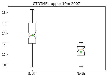
Comparing two sample means (another example)
The following shows the same calculations for temperature. In this case, the null hypothesis can be rejected at the 95% confidence level, and the 95% confidence intervals for the model slope do not overlap with zero.
plt.figure()
plt.boxplot([df07surf['CTDTMP'][iisouth],df07surf['CTDTMP'][iinorth]],
            labels=['South','North'],showmeans=True,notch=True);
plt.title('CTDTMP - upper 10m 2007')
Text(0.5, 1.0, 'CTDTMP - upper 10m 2007')
stats.ttest_ind(df07surf['CTDTMP'][iinorth],df07surf['CTDTMP'][iisouth],equal_var=True)
Ttest_indResult(statistic=-7.375689840798797, pvalue=1.4522086213500351e-11)
stats.ttest_ind(df07surf['CTDTMP'][iinorth],df07surf['CTDTMP'][iisouth],equal_var=False)
Ttest_indResult(statistic=-9.799130523807385, pvalue=1.7823812194777424e-17)
res = smf.ols(formula="CTDTMP ~ is_northern", data=df07surf).fit()
res.summary()
| Dep. Variable: | CTDTMP | R-squared: | 0.286 |
|---|---|---|---|
| Model: | OLS | Adj. R-squared: | 0.280 |
| Method: | Least Squares | F-statistic: | 54.40 |
| Date: | Tue, 03 May 2022 | Prob (F-statistic): | 1.45e-11 |
| Time: | 19:03:39 | Log-Likelihood: | -310.63 |
| No. Observations: | 138 | AIC: | 625.3 |
| Df Residuals: | 136 | BIC: | 631.1 |
| Df Model: | 1 | ||
| Covariance Type: | nonrobust |
| coef | std err | t | P>|t| | [0.025 | 0.975] | |
|---|---|---|---|---|---|---|
| Intercept | 13.6931 | 0.236 | 57.959 | 0.000 | 13.226 | 14.160 |
| is_northern[T.True] | -3.1587 | 0.428 | -7.376 | 0.000 | -4.006 | -2.312 |
| Omnibus: | 4.510 | Durbin-Watson: | 0.191 |
|---|---|---|---|
| Prob(Omnibus): | 0.105 | Jarque-Bera (JB): | 4.064 |
| Skew: | -0.408 | Prob(JB): | 0.131 |
| Kurtosis: | 3.202 | Cond. No. | 2.42 |
Notes:
[1] Standard Errors assume that the covariance matrix of the errors is correctly specified.
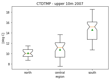
Comparing three sample means (another example)
We can also compare more than two means. This would be an ANOVA analysis, which can also be expessed as a linear model.
Create a categorical variable for the region
We will divide the data into three categories: north if the Columbia River, between the Columbia River and Golden Gate, and south of the Golden Gate.
# create a new variable called "region" with no values
df07surf = df07surf.assign(region = [None]*len(df07surf))
df07surf['region']
22      None
46      None
71      None
95      None
151     None
        ...
2275    None
2287    None
2310    None
2334    None
2335    None
Name: region, Length: 138, dtype: object
# assign string values to region based on latitude
northern = (df07surf['LATITUDE'] > 46.2)
central = (df07surf['LATITUDE'] <= 46.2) & (df07surf['LATITUDE'] >= 37.8)
southern = (df07surf['LATITUDE'] < 37.8)

df07surf.loc[northern,'region'] = 'north'
df07surf.loc[central,'region'] = 'central'
df07surf.loc[southern,'region'] = 'south'
df07surf['region']
22      north
46      north
71      north
95      north
151     north
        ...
2275    south
2287    south
2310    south
2334    south
2335    south
Name: region, Length: 138, dtype: object
Box plot
plt.figure()
plt.boxplot([df07surf['CTDTMP'][df07surf['region']=='north'],
             df07surf['CTDTMP'][df07surf['region']=='central'],
             df07surf['CTDTMP'][df07surf['region']=='south']],
            labels=['north','central','south'],showmeans=True,notch=True);
plt.title('CTDTMP - upper 10m 2007')
plt.ylabel('[deg C]')
plt.xlabel('region')
Text(0.5, 0, 'region')
Analysis
Since we have three groups, we can perform a classic Fisher ANOVA on this data set, to test the null hypothesis of no difference.
pg.anova(data=df07surf,dv='CTDTMP',between='region')
| Source | ddof1 | ddof2 | F | p-unc | np2 | |
|---|---|---|---|---|---|---|
| 0 | region | 2 | 135 | 86.688737 | 6.087664e-25 | 0.562225 |
However, looking at the box plot, it appears that the groups do not have equal variances (heteroscedesticity). This suggests that a Welch ANOVA may be more appropriate.
pg.welch_anova(data=df07surf,dv='CTDTMP',between='region')
| Source | ddof1 | ddof2 | F | p-unc | np2 | |
|---|---|---|---|---|---|---|
| 0 | region | 2 | 79.857577 | 117.8407 | 1.489427e-24 | 0.562225 |
Both have very low p-values. Now we move on to a post-hoc test. Which post-hoc test to use? The Tukey test is a good choice for the classic ANOVA because it corrects for pairwise comparisons. However, it assumes equal variances. A Games-Howell post-hoc test is preferable in this case.
pg.pairwise_gameshowell(data=df07surf,dv='CTDTMP',between='region')
| A | B | mean(A) | mean(B) | diff | se | T | df | pval | hedges | |
|---|---|---|---|---|---|---|---|---|---|---|
| 0 | central | north | 10.791951 | 10.124478 | 0.667473 | 0.320915 | 2.079905 | 60.998772 | 0.102548 | 0.535267 |
| 1 | central | south | 10.791951 | 14.616919 | -3.824968 | 0.361271 | -10.587518 | 95.679603 | 0.001000 | -2.047561 |
| 2 | north | south | 10.124478 | 14.616919 | -4.492441 | 0.296634 | -15.144727 | 88.746057 | 0.001000 | -3.586874 |
The p-values indicate that there is no statistically significant difference between the northern and central regions.
Ho does this compare to pairwise t-tests? The t-test indicates that there is a statistically significant difference (barely) at \(\alpha\)=0.05 between the northern and central regions.
pg.pairwise_ttests(data=df07surf,dv='CTDTMP',between='region')
| Contrast | A | B | Paired | Parametric | T | dof | alternative | p-unc | BF10 | hedges | |
|---|---|---|---|---|---|---|---|---|---|---|---|
| 0 | region | central | north | False | True | 2.079905 | 60.998772 | two-sided | 4.174356e-02 | 1.575 | 0.447480 |
| 1 | region | central | south | False | True | -10.587518 | 95.679603 | two-sided | 8.500978e-18 | 2.726e+15 | -1.944715 |
| 2 | region | north | south | False | True | -15.144727 | 88.746057 | two-sided | 2.478834e-26 | 4.026e+23 | -2.401071 |
We can also use statsmodels to perform this test as a linear model. Note that the F-statistic and Prob (F-statistic), a.k.a. p-value, are the same as the classic ANOVA.
The regression coefficients in this case can be thought of as pairwise comparisons with the central region. Note that the confidence intervals of the regression coefficient with the north region overlap with zero.
pg.homoscedasticity(data=df07surf,dv='CTDTMP',group='region')
| W | pval | equal_var | |
|---|---|---|---|
| levene | 9.765584 | 0.000109 | False |
res = smf.ols(formula="CTDTMP ~ region", data=df07surf).fit()
res.summary()
| Dep. Variable: | CTDTMP | R-squared: | 0.562 |
|---|---|---|---|
| Model: | OLS | Adj. R-squared: | 0.556 |
| Method: | Least Squares | F-statistic: | 86.69 |
| Date: | Tue, 03 May 2022 | Prob (F-statistic): | 6.09e-25 |
| Time: | 19:03:39 | Log-Likelihood: | -276.85 |
| No. Observations: | 138 | AIC: | 559.7 |
| Df Residuals: | 135 | BIC: | 568.5 |
| Df Model: | 2 | ||
| Covariance Type: | nonrobust |
| coef | std err | t | P>|t| | [0.025 | 0.975] | |
|---|---|---|---|---|---|---|
| Intercept | 10.7920 | 0.284 | 37.991 | 0.000 | 10.230 | 11.354 |
| region[T.north] | -0.6675 | 0.474 | -1.409 | 0.161 | -1.605 | 0.270 |
| region[T.south] | 3.8250 | 0.354 | 10.801 | 0.000 | 3.125 | 4.525 |
| Omnibus: | 8.796 | Durbin-Watson: | 0.310 |
|---|---|---|---|
| Prob(Omnibus): | 0.012 | Jarque-Bera (JB): | 4.392 |
| Skew: | -0.204 | Prob(JB): | 0.111 |
| Kurtosis: | 2.227 | Cond. No. | 4.28 |
Notes:
[1] Standard Errors assume that the covariance matrix of the errors is correctly specified.