Filtering and Convolution
Contents
Filtering and Convolution
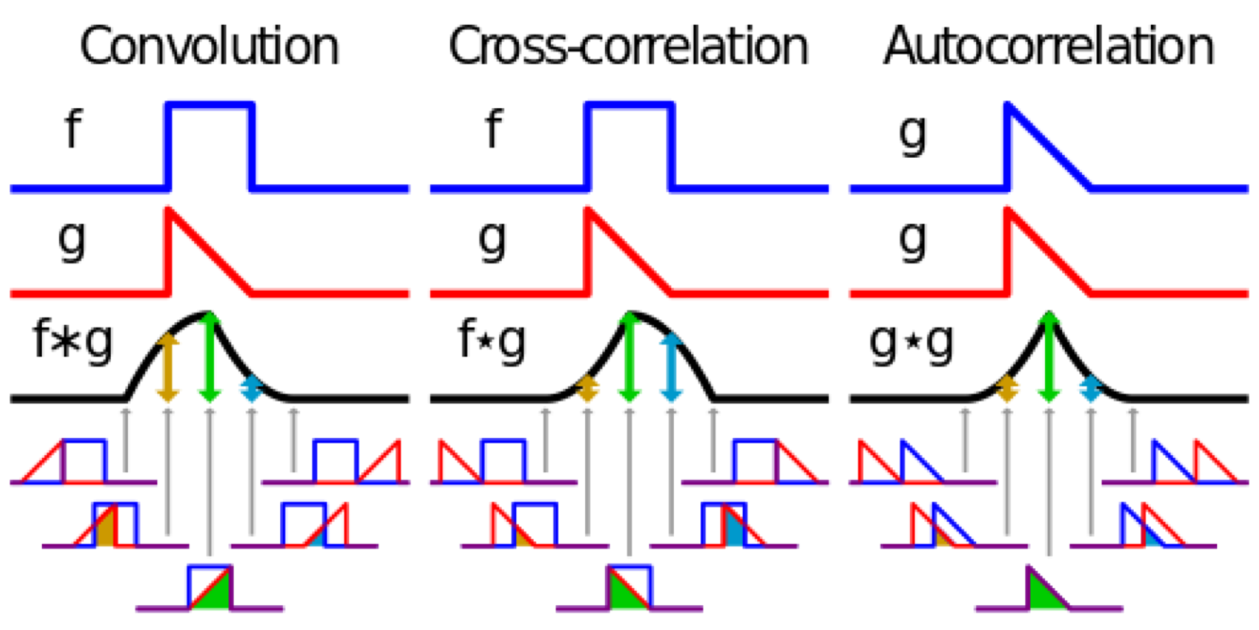
Convolution is a process of blending two functions together to create a third. The convolution of two functions \(f\) and \(g\) is symbolized mathematically as \((f * g)\).
Convolution steps
For each point in \(f\):
Flip \(g\) around
Take product of \(f\) and \(g\) at all overlapping location times
Add the resulting values together
Move on to next point in \(f\), repeat for different lag between \(f\) and \(g\)
This process is very similar to the procedures for cross-covariance of two functions \(f\) and \(g\), and auto-covariance of a single function \(g\) with itself.
source: https://en.wikipedia.org/wiki/Convolution
Expressing this procedure mathematically for two time series \(f(t)\) and \(g(t)\):
\(f\) has M samples, \(f_k\) where k = 1,2,3…M
\(g\) has N samples, \(g_i\) where i = 1,2,3…N
\( (f * g)_j = \sum_{k=1}^M g_{j-k} f_k \)
The resulting function has N+M-1 points.
Filtering
One of the common applications of convolution is smoothing data. Smoothing is used in time series analysis and image analysis to suppress noise or high-frequency variability. Another term for smoothing is low-pass filter becuase it suppresses high-frequency variability and allows low-frequency variability to pass through.
One of the most common and intuitive smoothing operations is the running Average (or Box Car filter). This involves taking the average over a certain block (30 hrs, 5 days … etc), then moving forward in time and repeating the same process for the next segment of data.
Filtering is a type of convolution where
\(f\) is a time series (observations)
\(g\) is a set of weights (filter)
For a running average, the weights in \(g\) are all identical and sum to one. If you plot the weights, the look like a rectangle, or “box car” shape.
Another common filtering method is the Hanning filter, which is a raised cosine function. All the values are positive (and sum to 1). This weights nearby points more than those that are farther away. Choosing the best filter for a certain situation is a major topic in digital signal processing.
What makes an ideal low pass filter?
Note: Images in this section come from the excellent source at http://www.labbookpages.co.uk/audio/firWindowing.html
For white noise (equal energy at all frequencies)
all energy in low frequencies (pass band) retrained
all energy in high frequencies (stop band) removed
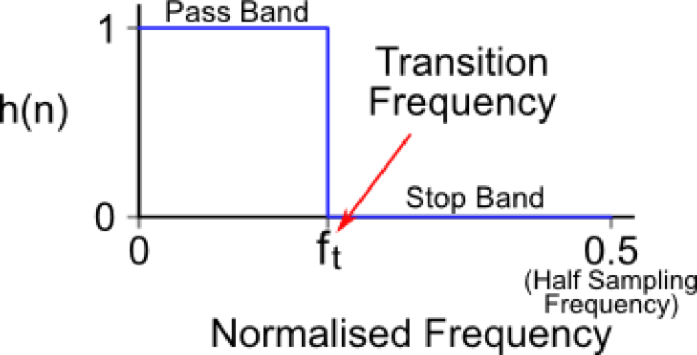
Image source: http://www.labbookpages.co.uk/audio/firWindowing.html
Ideal filter
Assuming an infinite time series, the filter would look like a sinc function:
sinc function is the FFT of a step function
convolving the sinc function with an infinitely long time series of white noise would give the step function in frequency content shown above
A sinc function would require an infinite number of weights (this is NOT practical)
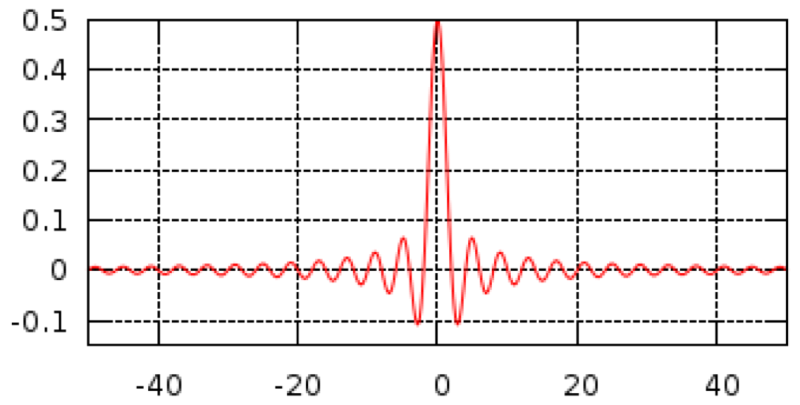
Image source: http://www.labbookpages.co.uk/audio/firWindowing.html
Practical filter
Ideal filter tapered off a the edges with a window
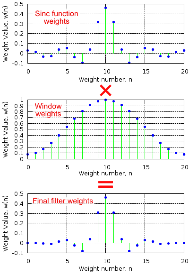
Image source: http://www.labbookpages.co.uk/audio/firWindowing.html
__ Spectral characteristics of filters __
Spectrum of white nose using this approach with two window types (box car and Hamming):
Ripples in frequency response of rectangular box car window (spectral leakage)
Hamming window has less ripples but a broader transition range (trade-off)
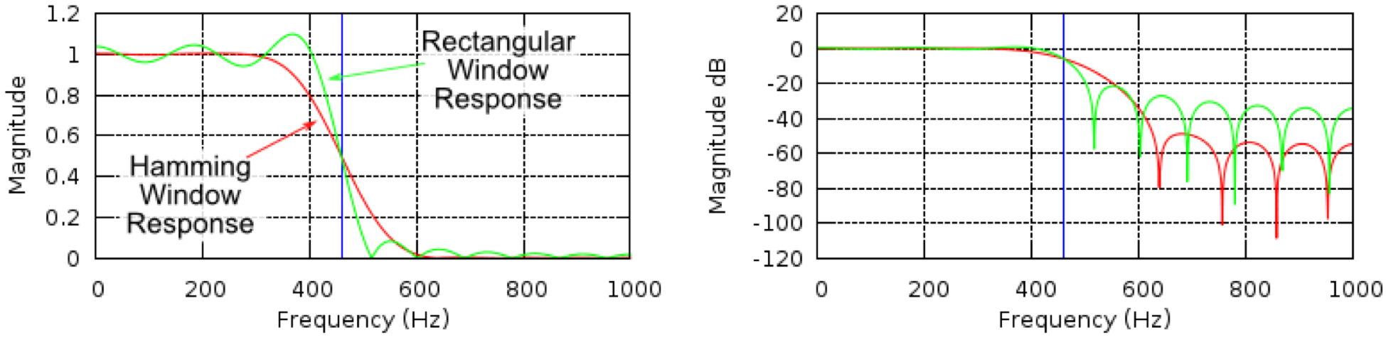
Image source: http://www.labbookpages.co.uk/audio/firWindowing.html
__dB - decibels __: logogrithmic unit used to describe attenuation (reduction of energy)
$\( dB = 10 \log_{10}\left(\frac{A^2}{A_0^2}\right) \)\( Where \) A_0 $ is a reference amplitude
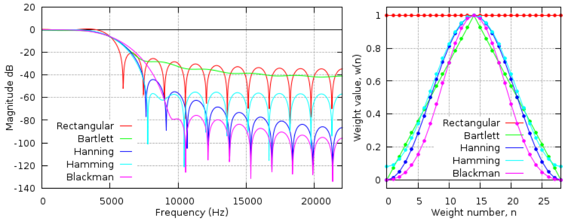
Image source: http://www.labbookpages.co.uk/audio/firWindowing.html
Common oceanographic filters
Cosine-Lanczos Filter
“Lancz7” filter: designed to filter out energy at diurnal and tidal fequencies
Half amplitude period = 34.29 hours
Half amplitude frequency = 0.7 cpd


Take Home Points: filtering
Boxcar filters (running averages) are simple but not very effective
A normalized Hanning window improves on the boxcar by soothing out the abrupt edges
More sophisticated filters (e.g. cosine-Lanczos) get closer to an ideal spectral response but require a large number of weights; not practical for shorter time series
Practical implementation
See example using data from the Elkhorn Slough LOBO mooring