NDBC data - analysis of wind vector time series¶

This notebook demonstrates common time series analysis techniques with a two-dimensional data set: wind velocity from a meteorological buoy offshore of Monterey Bay. The buoy is maintained by the National Data Buoy Center (NDBC).

The goal of this analysis is to rotate the wind data into an alongshore component (the wind blowing parallel to shore) and a cross-shore component (the wind blowing perpendicular to shore). This is useful because it is the alongshore component of wind stress that is responsible for coastal upwelling.

Functions are provided for analysis routines that are useful for a wide range of data sets. They are based on functions in a larger package located at https://github.com/physoce/physoce-py.

The example here is for wind data, but the same techniques can also be applied to ocean currents or any type of vector time series. As you go through the tutorial, try the exercises to check your understanding.

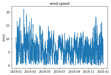
Working with vector data¶

Vectors, like wind velocity, are characterized by a magnitude and direction. Scalars, like temperature, only have a magnitude. Vectors can be described in different ways. For example, instead of speed and direction, we can describe a wind vector in terms of its eastward and northward components.

Calculating vector components¶

NDBC provides data on wind speed and direction. Following typical meteorological convention, the direction describes the direction the wind is blowing from, clockwise from true north. We can convert the data to eastward and northward components.

The eastward component describes how hard the wind is blowing towards the east. We will call this the \(u\) component, where positive \(u\) represents wind blowing toward the east and negative \(u\) represents wind blowing toward the west.

Similarly, the northward component describes how hard the wind is blowing towards the north. We will call this the \(v\) component, where positive \(v\) represents wind blowing toward the north and negative \(v\) represents wind blowing toward the south.

The function wind_uv_from_spddir converts wind vectors from speed and direction, as reported by NDBC, to eastward and northward components.

def wind_uv_from_spddir(wspd,wdir):
    '''Convert wind speed and direction to eastward and northward components.
    
    Inputs
    wspd - wind speed
    wdir - wind direction (wind is blowing FROM this direction, 
                           clockwise from true north)
    
    Output:
    u - eastward velocity component (TOWARDS the east)
    v - northward velocity component (TOWARDS the north)
    '''
    
    theta = np.array(wdir) # direction CW from true north
    theta = theta*np.pi/180. # convert to radians
    x = -np.sin(-theta)
    y = np.cos(-theta)
    theta_cart = np.arctan2(y,x) # direction CCW from east (Cartesian)
    u = -wspd*np.cos(theta_cart) # eastward component
    v = -wspd*np.sin(theta_cart) # northward component
    
    return u,v

ds['wind_east'],ds['wind_north'] = wind_uv_from_spddir(ds['wind_spd'],ds['wind_dir'])

ds['wind_east']

<xarray.DataArray 'wind_east' (time: 14855)>
array([0.17103359, 0.51289238, 1.84067075, ..., 2.58021354, 3.0564969 ,
       3.18198052])
Coordinates:
  * time       (time) datetime64[ns] 2019-01-01T00:50:00 ... 2019-12-31T23:50:00
    latitude   float32 36.78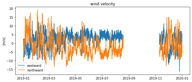
    longitude  float32 -122.4

Plot the vector components¶

Plot the time series of eastward velocity and northward velocity (time on the x-axis, both eastward and northward velocity on the y-axis).

plt.figure(figsize=(10,4))
plt.plot(ds['time'],ds['wind_east'])
plt.plot(ds['time'],ds['wind_north'])
plt.ylabel('[m/s]')
plt.title('wind velocity')
plt.legend(['eastward','northward'])

<matplotlib.legend.Legend at 0x7fdf516e3610>

Exercise¶

Identify a time when wind is blowing from the northwest and towards the southeast. This direction is favorable for upwelling along the California coast.

(insert text here)

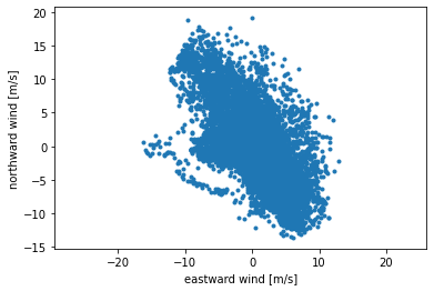
Alignment of wind velocity¶

By plotting eastward wind vs. northward wind, we can see that the wind off Monterey Bay tends to blow towards the southeast (upwelling-favorable) or towards the northwest (downwelling-favorable). This is because the wind tends to be steered parallel to the local coastline by coastal mountain ranges along the west coast.

plt.figure()
plt.plot(ds['wind_east'],ds['wind_north'],'.')
plt.xlabel('eastward wind [m/s]')
plt.ylabel('northward wind [m/s]')
plt.axis('equal'); # make the scale equal on the x and y axes

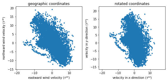
Coordinate system rotation¶

Rotating wind stress vectors¶

The northward and eastward components of wind stress are not always the most useful for studying upwelling. It is the alongshore component of wind stress (the component parallel to shore) that is most important for upwelling. The direction parallel to shore is not always conveniently aligned in the north-south or east-west directions.

To calculate the alongshore component of wind stress, the vectors are rotated from geographic coordinates (east and north) to “natural” coordinates (cross-shore and alongshore). The rot function rotates vectors to a new coordinate system defined by the user.

def rot(u,v,theta):
    """
Rotate a vector counter-clockwise OR rotate the coordinate system clockwise.
Usage:
ur,vr = rot(u,v,theta)
Input:
u,v - vector components (e.g. u = eastward velocity, v = northward velocity)
theta - rotation angle (degrees)
Output:
ur,vr - rotated vector components
Example:
rot(1,0,90) returns (0,1)
    """

    w = u + 1j*v             # complex vector
    ang = theta*np.pi/180    # convert angle to radians
    wr = w*np.exp(1j*ang)    # complex vector rotation
    ur = np.real(wr)         # return u and v components
    vr = np.imag(wr)
    return ur,vr

See what happens when the vectors are rotated 20 degrees clockwise.

rotation_angle = -20
ds['wind_x'],ds['wind_y'] = rot(ds['wind_east'],ds['wind_north'],rotation_angle)

plt.figure(figsize=(8,4))
plt.subplot(121)
plt.plot(ds['wind_east'],ds['wind_north'],'.')
plt.axis('equal')
plt.xlabel('eastward wind velocity ($\\tau^{se}$)')
plt.ylabel('northward wind velocity ($\\tau^{se}$)')
plt.title('geographic coordinates')

plt.subplot(122)
plt.plot(ds['wind_x'],ds['wind_y'],'.')
plt.axis('equal')
plt.xlabel('velocity in $x$-direction ($\\tau^{sx}$)')
plt.ylabel('velocity in $y$-direction ($\\tau^{sy}$)')
plt.title('rotated coordinates')
plt.tight_layout()

Exercise¶

Modify the rotation_angle variable above and re-run the analysis. What angle makes the wind stress most aligned along the \(y\) axis? What angle makes the wind stress most aligned along the \(x\) axis?

Principal axis angle¶

Instead of trial and error, a principal axis analysis can be used to find the angle along which the wind stress is aligned. On the west coast, this typically corresponds with the local coastline. On the east coast, this is not necessarily case.

The princax function can be used to find the pricipal axis angle. The variance of the data is maximized along this axis.

def princax(u,v=None):
    '''
Principal axes of a vector time series.
Usage:
theta,major,minor = princax(u,v) # if u and v are real-valued vector components
    or
theta,major,minor = princax(w)   # if w is a complex vector
Input:
u,v - 1-D arrays of vector components (e.g. u = eastward velocity, v = northward velocity)
    or
w - 1-D array of complex vectors (u + 1j*v)
Output:
theta - angle of major axis (math notation, e.g. east = 0, north = 90)
major - standard deviation along major axis
minor - standard deviation along minor axis
Reference: Emery and Thomson, 2001, Data Analysis Methods in Physical Oceanography, 2nd ed., pp. 325-328.
Matlab function: http://woodshole.er.usgs.gov/operations/sea-mat/RPSstuff-html/princax.html
    '''

    # if one input only, decompose complex vector
    if v is None:
        w = np.copy(u)
        u = np.real(w)
        v = np.imag(w)

    # only use finite values for covariance matrix
    ii = np.isfinite(u+v)
    uf = u[ii]
    vf = v[ii]

    # compute covariance matrix
    C = np.cov(uf,vf)

    # calculate principal axis angle (ET, Equation 4.3.23b)
    theta = 0.5*np.arctan2(2.*C[0,1],(C[0,0] - C[1,1])) * 180/np.pi

    # calculate variance along major and minor axes (Equation 4.3.24)
    term1 = C[0,0] + C[1,1]
    term2 = ((C[0,0] - C[1,1])**2 + 4*(C[0,1]**2))**0.5
    major = np.sqrt(0.5*(term1 + term2))
    minor = np.sqrt(0.5*(term1 - term2))

    return theta,major,minor

Use this function on the wind stress data.

theta,major,minor = princax(ds['wind_east'],ds['wind_north'])

Rotate the wind data based on the principal axis angle. Note that it is common among oceanographers on the west coast to align the alongshore coordinate with the \(y\)-axis, but this is up to you.

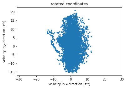
ds['wind_x'],ds['wind_y'] = rot(ds['wind_east'],ds['wind_north'],-theta-90)

plt.figure()
plt.plot(ds['wind_x'],ds['wind_y'],'.')
plt.axis('equal')
plt.xlabel('velocity in $x$-direction ($\\tau^{sx}$)')
plt.ylabel('velocity in $y$-direction ($\\tau^{sy}$)')
plt.title('rotated coordinates')

Text(0.5, 1.0, 'rotated coordinates')

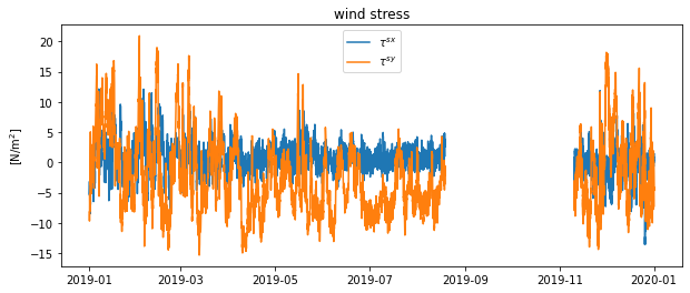
Plot the time series. The negative values of the alongshore wind stress (\(\tau^{sy}\)) indicate upwelling-favorable winds. The positive values indicate downwelling favorable winds.

plt.figure(figsize=(10,4))
plt.plot(ds['time'],ds['wind_x'])
plt.plot(ds['time'],ds['wind_y'])
plt.ylabel('[N/m$^2$]')
plt.title('wind stress')
plt.legend(['$\\tau^{sx}$','$\\tau^{sy}$'])

<matplotlib.legend.Legend at 0x7fdf52a07d90>

Exercise¶

Apply this same analysis to another NDBC buoy on the west coast.

Find the buoy ID number using the map interface at https://www.ndbc.noaa.gov/
In the ncfile variable above, replace 46042 with the new buoy ID number.
Identify a time when the wind is favorable for upwelling.
What rotation angle did you use?

Data Analysis Techniques in Marine Science

NDBC data - analysis of wind vector time series

Contents

NDBC data - analysis of wind vector time series¶

Outline¶

Load data and packages¶

Data source¶

Load Python packages¶

Load wind data¶

Data structure¶

Labeled arrays¶

Exercise¶

Time series plots¶

Exercise¶

Working with vector data¶

Calculating vector components¶

Plot the vector components¶

Exercise¶

Alignment of wind velocity¶

Coordinate system rotation¶

Rotating wind stress vectors¶

Exercise¶

Principal axis angle¶

Exercise¶