Example: Modeling exponential growth
Contents
Example: Modeling exponential growth
The goal of this exerice is to find the parameters of an exponential fit of US population growth with time
where \(y\) is population and \(t\) is time in years.
Data for this exercise is located in a text file at data/uspopulation
This exercise is based on Chapter 38 of Shapiro, B. E. (2016) Scientific Computation: Python Hacking for Math Junkies, Sherwood Forest Publishing.
import numpy as np
import pandas as pd
import matplotlib.pyplot as plt
from scipy import stats
First, read in the data and put into variables that are easy to remember and type.
df = pd.read_csv('data/uspopulation/us-population.txt',header=2)
yr = df['YR']
pop = df['USPOP']
Since this example is focused on the US, create a new variable where the year is referenced to the founding of the US.
t = yr - 1776
logpop = np.log(pop)
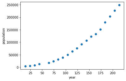
Plotting the data
plt.figure()
plt.plot(t,pop,'o')
plt.xlabel('year')
plt.ylabel('population')
Text(0, 0.5, 'population')
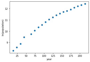
plt.figure()
plt.plot(t,logpop,'o')
plt.xlabel('year')
plt.ylabel('ln(population)')
Text(0, 0.5, 'ln(population)')
Exercises:
Estimate the parameters \(a_1\) and \(a_2\) is to performing a linear least-squares fit to the log-transformed data shown above. Note that log-transforming both sides of the first equation gives \(\ln(y) = \ln(a_1) + a_2 t\)
Plot the original data (not transformed) and the exponential fit using these parameters.
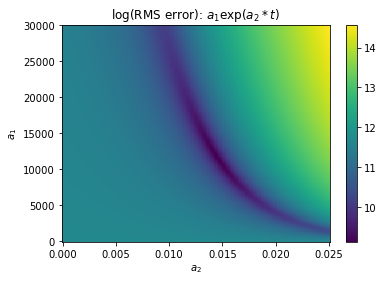
Visualizing the cost function
An extremely inefficient way of optimizing the parameters would be to try every possible combination of parameters within some range. This is called the “brute force” method because it relies on computer power rather than intelligence.
Even though it is inefficient, it is a good way to visualize the cost function in two dimensions.
# plot the (square root of) the cost function
# as a function of fit paramters
alla1 = np.linspace(0,3e4,200)
alla2 = np.linspace(0,0.025,200)

# pre-allocate error matrix
rms = np.nan*np.ones([len(alla1),len(alla2)])

# nested for loop
# go through each combination of parameter pairs in that range
# 200 x 200 = 40000 values
for ii,a1 in enumerate(alla1):
    for jj,a2 in enumerate(alla2):
        popfit = a1*np.exp(a2*t)
        rms[ii,jj] = np.sqrt(np.mean((popfit-pop)**2))

plt.figure()
plt.pcolor(alla2,alla1,np.log(rms),cmap='viridis')
#plt.plot(slope,np.exp(intercept),'ro')
plt.colorbar()
plt.title('log(RMS error): $a_1\exp(a_2*t)$')
plt.xlabel('$a_2$')
plt.ylabel('$a_1$')
Text(0, 0.5, '$a_1$')
Non-linear optimization
The first step in this process is to define the function that you want to fit to data.
def exponential_growth(t,a1,a2):
    '''inputs:
    t - vector of times
    a1 - initial population at time 0
    a2 - specific growth rate

    returns: modeled population based on exponential growth
    '''
    # insert code here
    return f
help(exponential_growth)
Help on function exponential_growth in module __main__:

exponential_growth(t, a1, a2)
    inputs:
    t - vector of times
    a1 - initial population at time 0
    a2 - specific growth rate

    returns: modeled population based on exponential growth
fvalues = exponential_growth(np.array([0,1]),10,1)
print(fvalues)
---------------------------------------------------------------------------
NameError                                 Traceback (most recent call last)
/var/folders/67/t9t76vyd78qgn_kwjr1_76yr0000gn/T/ipykernel_74375/2852909755.py in <module>
----> 1 fvalues = exponential_growth(np.array([0,1]),10,1)
      2 print(fvalues)

/var/folders/67/t9t76vyd78qgn_kwjr1_76yr0000gn/T/ipykernel_74375/3487471894.py in exponential_growth(t, a1, a2)
      8     '''
      9     # insert code here
---> 10     return f

NameError: name 'f' is not defined
The scipy.optimize library can be used to find the unknown coefficients. The curve_fit function is especially good at find the minima of cost functions. It needs to have 1) the function being fit (exponential_growth1) and 2) the data values (t,pop). It also really helps to have a good initial guess for the parameter values (p0).
from scipy.optimize import curve_fit
popt,pcov = curve_fit(exponential_growth,t,pop,p0=[]) # insert first guess for p0
The first variable in the output (popt) is the two coefficients that give the optimal fit to the data.
popt
array([1.17678552e+04, 1.45465803e-02])
Estimating error of coefficients
The second variable in the output (pcov) is the error covariance matrix.
pcov
array([[ 1.59526049e+06, -7.10599907e-01],
       [-7.10599907e-01,  3.26096426e-07]])
The diagonal elements of the covariance matrix can be thought of as the variance that there would be in the coefficient if you resampled many times and repeated the fit procedure. This could be estimated from the data using subsets of the data.
The square root of the diagonals are called the standard errors of the parameter estimates (e.g. \(\sigma_a\) for parameter estimate \(\hat{a}\)). If you resampled many times, and the errors are normally distributed, then about 68% of the parameter estimates would fall in the interval \(\hat{a}-\sigma_a < a < \hat{a}+\sigma_a\). Confidence intervals can be computed using the standard error and the t-statistic.
err = np.sqrt(np.diag(pcov))
print(err)
[1.26303622e+03 5.71048533e-04]
The diagonals of the error covariance matrix decribe correlations that occur in estimates of the different parameters. For example, if you resample many times, does parameter \(a\) usually increase when parameter \(b\) increases? If so, this means that the parameters covary when resampling, and this would result in a positive error covariance term.
plt.figure()
plt.pcolor(alla2,alla1,np.log(rms),cmap='viridis')
plt.colorbar()
#plt.plot(slope,np.exp(intercept),'ro')
#plt.plot(popt[1],popt[0],'rs')
plt.title('log(RMS error): $a_1\exp(a_2*t)$')
plt.xlabel('$a_2$')
plt.ylabel('$a_1$')

plt.plot([popt[1]-err[1],popt[1]+err[1]],
         [popt[0],popt[0]],'r-')
plt.plot([popt[1],popt[1]],
         [popt[0]-err[0],popt[0]+err[0]],'r-')
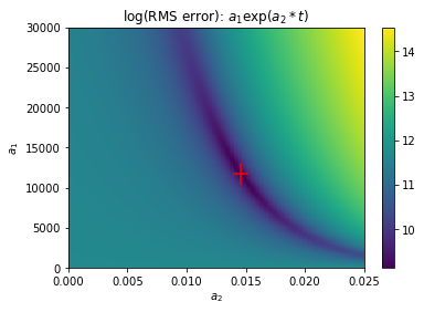
Plotting the parameter estimate on the map of the cost function shows that the nonlinear optimization procedure (square) succeeds in finding the minimum of the cost function, thus minimizing the sum of squared differences between the data values and corresponding model values.
The standard errors can be visualized in this map of the cost function. The height and width of the red error bars are determined by the standard errors of the coefficients.
Excercises
Plot the parameters obtained from the linear regression of the log-transformed data on the cost function map.
Use the optimization techniques described above to fit an exponential curve to the data from phytoplankton growth experiments
Write a function that can be used to fit an exponential curve to any data set, and return the standard error of the coefficients.